
Overview
Several weeks ago the data visualization community broke into justified outrage over an inexcusably misleading dual-axis chart from Americans United for Life. I plan to write an article about this and other “ethically wrong” visualizations in a few weeks but in the meantime I encourage you to read these excellent posts from Alberto Cairo and Emily Schuch, as well as this discussion from Politifact.
Around the same time these posts appeared I came across a “Viz of the Day” dashboard from Emily Le Coz that accompanied a lengthy article in the Daytona Beach News-Journal. The dashboard contained several visualizations but the one that caught my eye was this dual axis chart.

Figure 1 — Infographic showing that as the number of firefighters has increased over the past 30 years, the number of fire-related deaths has decreased.
I engaged in an interesting Twitter discussion about this graphic with Alberto Cairo, Jorge Camoes, and Noah Illinsky. I’ll get into that discussion in a bit (and point out some troubling problems with the visualization) but first want to discuss the use case for dual axis charts.
Why use dual axis charts
There are several reasons to use a dual axis chart (e.g., a Pareto chart that shows individual values along with the cumulative percent) but the primary use case is when you want to compare two completely different measures and see if there is any noteworthy relationship between the two measures. Consider the example below that shows cyclical sales data for a retail store (bars) and the number of orders placed each month (line).
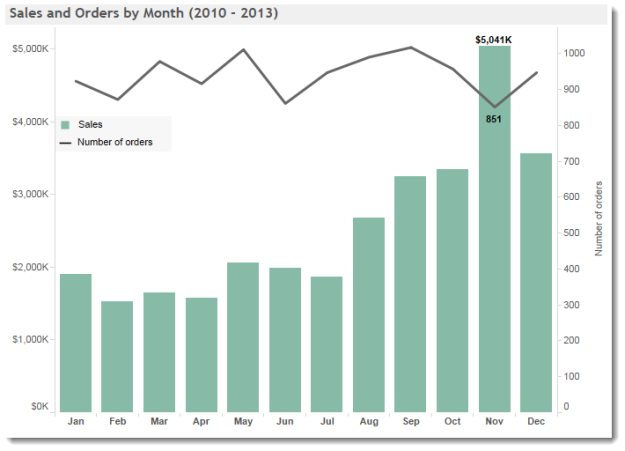
Figure 2 — Dual axis chart comparing sales and orders by month.
The surprising result is that while November is historically the strongest month for sales ($5M from 2010 to 2013) the total number of orders placed in November is the lowest of any month. And yes, I checked to make sure that this was true of all years and not one crazy blowout year.
I think this dual axis combination chart (where we show bars and a line) makes it easy to see there is something very interesting about November. The low number of orders combined with the high sales – something that is easy to see – means that we either sold more items per order or more expensive items per order.
So, what’s wrong with the firefighter example?
Given that dual axis charts can be so useful I wondered why I had problems with the Firefighter example. Fortunately, the author made the dashboard downloadable from Tableau public so I was able to see how it was put together.
Cutesy icons set the wrong tone for the piece
My first problem was with the firefighter hat and skull-and-crossbones icons.

Figure 3 — Icons representing firefighters and civilian deaths.
In my opinion (and it is just an opinion) I thought this “cartoonified” the visualization. I would much prefer to see either a simple color legend or a label next to both lines.
The author exaggerates the changes over time
A much more troubling issue is that the author uses a fixed Y-axis that exaggerates the changes over time. The author also fails to show the axis labels so we can’t see that the axis doesn’t start at zero.
Consider the dashboard below that shows the original visualization on the left with an accurate visualization on the right.
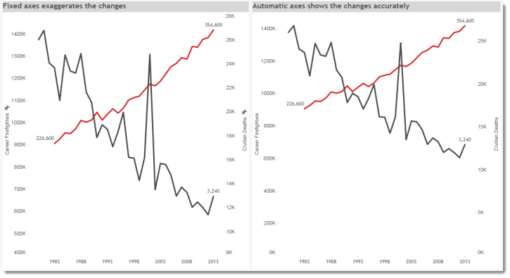
Figure 4 — Comparison of fixed axis vs. automatic axis charts. Note that the axis uses a SUM() function while the label is using AVERAGE(). The data is repeated three times in the data source which is why the author needs to use AVERAGE(). Yes, the axis should use AVERAGE() as well but the relative positioning of the elements is the same with SUM() so this causes no harm.
Because the author fixed the Y-axis rather than starting from zero, the slope of the lines is exaggerated. While this does not alter what is in fact a noteworthy observation, whenever I see this type of “rigging” it makes me question the validity of any and all parts of the story. That is, even though I don’t think the exaggeration was an intentional attempt to dramatize the difference, seeing this in play will make me question everything that the author and the publication now publishes.
Am I being too hard on the author? I don’t think so as anything that’s published as a “viz of the day” and accompanies a high-profile news article should get a lot more scrutiny than just any old Tableau Public visualization. While I don’t feel mislead by the overstated changes, I do wonder at what point does a viz cross the line into TURD territory (Truly Unfortunate Representation of Data)? We’ll save that discussion for a later post.
Different approaches
Combination area and line chart
After adjusting the axis I still wondered if having two line charts was causing unnecessary confusion. In my first makeover attempt I tried combining an area graph with a line chart, as shown here.

Figure 5 — First makeover attempt. A dual axis chart using an area chart for firefighters and a line chart for civilian deaths.
While using two different chart types made it easier to see that I was comparing two different measures, I didn’t love the chart and sought alternatives.
Connected Scatterplots
On Twitter Jorge Camoes offered this connected scatterplot.

Figure 6 — Jorge Camoes’ connected scatterplot. Notice that the axes do not start at zero but that the axes labels are at least visible.
In a connected scatterplot the path the line takes represents the year. This is why the line folds back on itself from time to time (more on this in a moment). Camoes also “normalized” the data using an index so that both civilian deaths and number of firefighters start at a value of 100.
I like this visualization very much but fear that many people won’t understand the index value of 100 so I tried my own connected scatterplot, shown below.
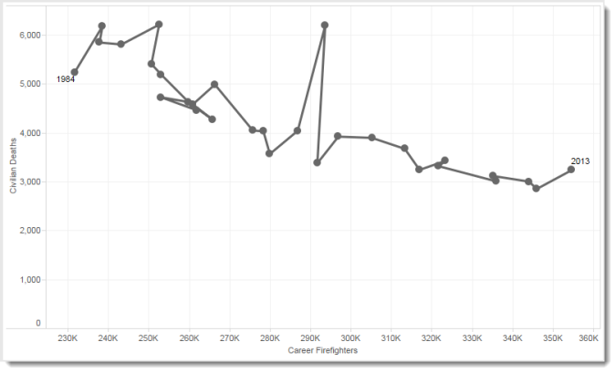
Figure 7 — Connected scatterplot with regular vs. normalized values. Notice that the X-axis does not start at zero but that the axes labels are visible.
Before anyone cries foul about the X-axis, here’s a version with the axis starting at zero.
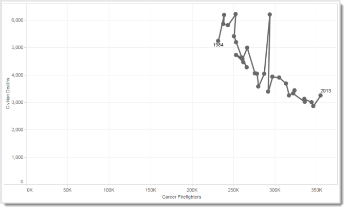
Figure 8 — Connected scatterplot with both axes starting at zero. This may be why Camoes normalized the data although his chart doesn’t start at zero, either.
I think starting the x-axis at zero obscures the relationship but that’s not what makes me question using this approach. My problem is that many people will have a hard time understanding how the line “works”, as it were. This is because whenever we see a line chart that involves time we come to expect marks on the left of the chart to show older dates and marks on the right to show newer dates. In other words, we expect the chart to behave like this.

Figure 9 – Since grade school we’ve been indoctrinated to expect earlier dates to the left and later dates to the right.
With a connected scatterplot the X-axis is “owned” by an independent measure so we have to adjust our perception to see that sometimes a later year will appear to the left of an earlier year, as shown below.

Figure 10 — Connected scatterplot with marks showing all years.
Notice how 1986 appears to the left of 1985 and 1989 appears to the left of 1988. Unless you are used to this type of approach this can look very strange.
Keep it simple
After experimenting a bit more I decided to forgo the dual axis and connected scatterplots and fashioned this simpler narrative.

Figure 11 — Two separate charts yielding a simple and easy-to-follow narrative.
If you have what you think is a better approach I would love to see it. If you’re using Tableau you can download the packaged workbook with the original dashboard and various makeover attempts here.

