Finally, a good use for packed bubbles!
The Problem
I recently received a query from a client on how to compare responses to one question with responses to another question when both questions have possible LIkert values of 1, 2, 3, 4, and 5. That is, if you have a collection of questions like this:

How would you show response clusters when you compare “Good Job Skills” against “Likes the Beatles”?
This question is particularly applicable if you are a provider of goods and services and you want to see if there is alignment or misalignment between “how important is this feature” and “how satisfied are you with this feature”.
Note: There’s a Tableau forum thread that has been looking into this issue as well. Please see http://community.tableausoftware.com/thread/137719.
So, how can we fashion something that helps us understand the data?
Before we get into the nitty gritty here’s a screen shot of one of the approaches I favor. Have a look to determine if reading the rest of the blog post is worth the effort.

Still reading? Well, I guess it’s worth the effort.
The Traditional Scatterplot Approach
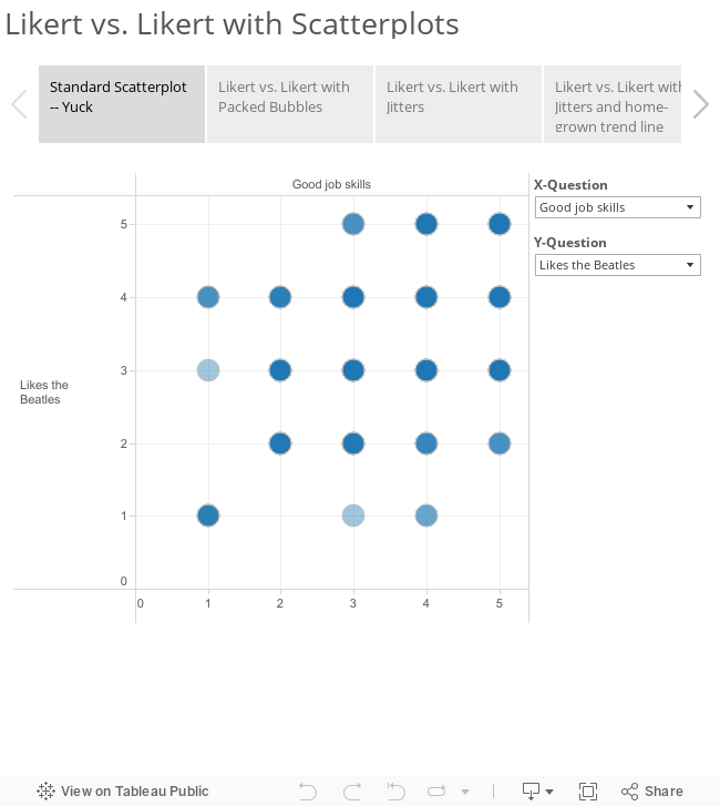
Consider the set up below where we see how Tableau would present the Likert vs. Likert results in a standard scatterplot.

So, what is going on here?
There are a total of nine Likert questions available from the X-Question and Y-Question parameter drop down list boxes. Our desire here is to allow us to compare any two of the nine at any time.
The “meat” of the visualization comes from the SUM(X-Value) on the columns shelf and SUM(Y-Values) on the rows shelf where X-Value and Y-Value are both defined as
IF [Wording]=[X-Question] then [Value]+1 END
This translates into “if the selected item from the list is the same as one of the questions you want to analyze, use the [Value] for that question”. Note that [Wording] is the same as [QuestionID] but with human readable values (e.g., “Likes the Beatles” instead of “Q52”)
We use [Value]+1 is because the Likert values are set to go from 0 to 4 instead of 1 to 5, and most people expect 1 to 5.
We can use SUM(X-Value) and SUM(Y-Value) because we have Resp ID on the Details shelf. This forces Tableau to draw a circle for every respondent. The problem is that we have overlapping circles and even with transparency you don’t get a sense of where responses cluster. Yes, it is possible with a table calculation to change the size of the circle based on count but we’ll I’ll provide what I think is a better approach below.
A note about the filters: The Question filter is there to constrain our view so that we only concern ourselves with Likert Scale questions. It isn’t necessary but is useful should we be experimenting with different approaches. The SUM(X-Value) and SUM(Y-Value) filters remove nulls from the view.
Packed Bubbles to the Rescue
I’m not a big fan of packed bubbles (see this post) but for this situation we can use them and get some great results, as shown below.

I’ve made a couple of changes to the traditional scatterplot visualization the most important being SUM(X-Value) and SUM(Y-Value) are now discrete and we get a trellised visualization instead of a continuous axis. Note that I had to change the sort order of the Y-axis elements so that they appear in reverse order (5 down to 1).
I got the packed bubbles by placing CNTD(Resp ID) on the size button. This assures that each bubble is the same size and triggers Tableau’s packing algorithm.
Note that I also added an on-demand “Drill down” so that you can color the circles by different demographic dimensions.
I’ve experimented with this with some large data sets and Tableau does a great job with packing the bubbles intelligently.
What About Trend Lines?
Since we are using discrete measures on the rows and columns shelves we cannot produce trend lines. When I first started this project I experimented with more traditional jittering and was able, with a fair amount of fuss and bother, to produce this.

A special thanks to Jeffrey Shaffer who provided a link on how to create pseudo-random numbers in Tableau (thank you, Josh Milligan).
I prefer the example that doesn’t require the jittering, but if you need to trend lines or if you prefer the jittered look I’ve included the example in the downloaded packaged workbook (see below).
It also occurred to me that the trend line would be based on the jittered values and not the actual values. The same workbook contains a “home grown” trend line based on the actual values (courtesy of Joe Mako). It turns out the jittered trend line is almost identical to the non-jittered trend line so I suspect you won’t need to take the “home grown” approach.
Update
I received a number of comments here and on LinkedIn about the “drill down / break down” capability and that it is hard to see the percentage of dots by category. For example, if you break down by generation do the dots for one generation cluster more in one part of the trellis than in others?
I thought that in this case having a different-colored bubble per category where the size of the bubble was proportionate to the percentage of responses within that category made sense.

I thought building this would be easy, but I needed to call in the heavy artillery (Joe Mako).
I’ll blog about the solution later. In the meantime the packaged workbook below contains this additional approach.