August 6, 2019
Overview

Since the release of The Big Book of Dashboards in the Spring of 2017 I’ve received a lot of requests to explain how to build the Churn dashboard in Tableau. I’m glad I waited to write the post as my friend and colleague Klaus Schulte came up with a considerably better way to both structure the data and craft the waterfall / line chart visualization.
I’ll write about one of several ways to build the view in a moment, but first let me make sure people understand the scenario and how the data needs to be structured.
Note: You can read the entire Churn dashboard chapter for free by clicking here.
Scenario and data set
Let’s say you need to track subscriber churn so that for each month you know how many people sign up for a service and how many people cancel, broken down by different divisions. Your source data might look like this in Excel.

Figure 1 — Twelve months of churn data in Excel.
Before we can do anything in Tableau we’re going to need to ditch the wide format and have a single date column. Using whatever tool you prefer (Alteryx, Easy Morph, Tableau Prep, or Tableau’s built-in pivoting feature, etc.) we need our source data to look like this.

Figure 2 — Reshaped data. We just need to know how many we gained and how many we lost for each division in each month. We’ll be able to calculate everything else in Tableau.
How the main view works
I experimented with several different GANTT chart approaches and will explain the technique that I think is easiest to understand. All the GANTT approaches require a little bit of “move the slider to the right until it looks right” uncertainty versus something that is “pixel perfect.” Klaus has developed a Polygon approach that’s “pixel perfect” but it does require more preparation work (and a lengthier blog post!)
Here’s the combined waterfall / jump line view.

Figure 3 — Waterfall chart with jump line overlaid.
We can see by (1) that we’re dealing with a dual axis chart, let’s separate this into two views and focus on the Month Offset component first, which is responsible for drawing the paired GANTT bars.
Understanding the GANTT bars

Figure 4 — What’s behind the GANTT chart. Note that SUM(Amount) is on detail so that the amount gained or lost for a month appears when the user hovers over a bar.
Month Offset (1) is a calculated field and is defined as follows.
   DATETRUNC('month',[Date]) +

   IF [Description]="Gained" THEN

     -[Offset]

   ELSE

     [Offset]

   END
This translates as “round the date to the nearest month, if we’re looking at gains, move the mark a little to the left (minus Offset) if we’re looking at losses, move the mark a little to the right (plus Offset).”
This is where things get a little wonky. Offset is a parameter and it’s currently set for 5.3. Why that number? Because combined with manually sizing the GANTT bar (2), it looks good.
Notice that the field [Description] is on color. This creates two separate marks: gray for “Gained” and red for “Lost”, for each month.
So, at this point we know that we have a pair of offset GANTT bars for each month. Where should the marks start (i.e., how high or low) and how tall should they be?
The field [Running SUM(Amount)] determines where the bars should start. This field is defined as follows.
RUNNING_SUM(SUM([Amount]))
This table calculation tells Tableau to add the current month to the sum of the previous months. It is critical that “compute using” be setup as follows.

Figure 5 — Make sure that the Description field isn’t first.
Actually, the only critical thing is that the [Description] field come after one of the date fields.
So, now we know where the GANTT bars need to start. How long should they be? This is determined by size (5) where we have the field SUM(-Amount).
Why the negative? That’s how GANTT bars work. You figure out where the end should be and then extend the marks down from where it should start.
Understanding the jump line chart

Figure 6 — What’s behind the jump line chart.
We start by placing the MONTH([Date]) as a continuous datavalue on columns (1). This will center our line chart (2) at the start of the month versus offsetting. Notice, too, that we have the same computation on the rows shelf, but we do not have a designation for color, so we get a single line chart, colored blue, that shows the overall running sum of net subscribers.
Clicking the Path button will reveal that we’re using a “Jump” line type (3).

Figure 7 — Specifying a “Jump” line type.
We specify a “Jump” type of line as we just want a horizontal line connecting the months and don’t need to draw vertical lines.
I think adding mark labels is optional, but if you do want them sure the labels (4) are right aligned along the bottom.

Figure 8 — Label settings.
The last step is to make this a dual axis chart and make sure the axes are synchronized.
Iterate, iterate, iterate
This single visualization – let along the entire dashboard – went through a lot of iterations. The version we published in the book looked like this.

Figure 9 — Original version of waterfall / line chart combo.
I recently flirted with a zig-zag chart that made it easy to go down the path of “this many people signed up, then this many people cancelled, then this many people signed up”, etc.

Figure 9 — Zig-zag chart. A little on the noisy side.
I think both the original and the zig-zag work, but I prefer the clean look of the jump line. Again, I very much appreciate Klaus showing me that I didn’t need to compute the net results for each month as a separate field in the source data and for coming up with the jump line technique. I think this is a good approach as the data prep is easy, the chart calculations are easy, and we have a clear and easy-to-understand viz.
Want to explore the complete dashboard and download it? Click here.
Click here to read Klaus Schulte’s blog post that explores his pixel-perfect polygon technique.